Extended Energy Conservation Law in Alloys: the Absence of Energy Non-Equilibrium

Choi, Myung Sik; Na, Han Gil; Jin, Changhyun; Lee, Kyu Hyoung

doi:2020.58.8.566

Abstract

Assuming that many of the materials produced in a non-equilibrium state remain unchanged, an extended space–energy conservation law was proposed based on the existing energy conservation law. In the present study, by analyzing the well developed equilibrium binary phase diagram of iron (Fe) – carbon (C), we show that energy non-equilibrium microstructures can appear as a part of the equilibrium between the space energy and the mass energy. The correlation between these two energies is objectively and logically explained via (1) one-to-one correspondences between the equilibrium and non-equilibrium phases based on the binary Fe–C phase diagram and (2) the heat-treated Fe–C phases with the spatial energy represented by temperature. Additionally, we found that the morphological and microstructural changes in non-equilibrium states could be consistently explained using the extended energy law as a major premise. This suggests that material factors such as size, distribution, and the shape of materials, which appear to have no energy transfer, are all formed to balance the energy equilibrium with the spatial energy surrounding the materials. Thus, an extended energy conservation law, which can control mass through space or vice versa, can provide a comprehensive logical framework for analyzing various unsolved physicochemical phenomena.

Key words: energy equilibrium, phase diagram, mass energy, space energy

1. Introduction

One of the most fundamental questions regarding matter, whether a new reaction will or will not occur, and how quickly it will occur, led to the emergence of thermodynamics [1,2]. At the basis of thermodynamics is the fact that all physicochemical reactions that occur between materials proceed in a manner that lowers their total energy; the larger the gradient, the faster the reaction proceeds. Moreover, these energies can have different forms, such as Helmholtz energy (F) [3], internal energy (U) [4], Gibbs energy (G) [5], enthalpy (H) [6], and external energy (PV) [7]. Most of these energies are not path functions, which depend on the path taken to reach a specific value, but are state functions that are not path dependant. A reaction between a reactant and product means that there is an energy non-equilibrium between them, which indicates that a dynamic energy transfer is required to reach an energy equilibrium. However, in the most cases, the understanding of a reaction is based on room temperature. That is, if the reference point is changed, all physicochemical reactions can reach energy equilibrium at every moment. Therefore, since energy equilibria based on different criteria are considerably different from each other, theoretically, an energy non-equilibrium cannot exist. This can be easily understood from the following example (Fig 1).

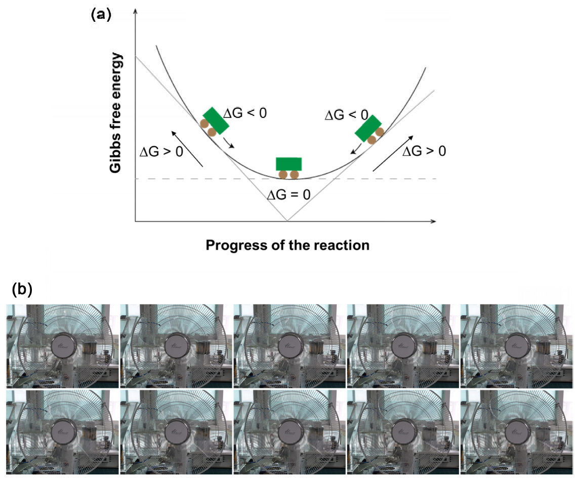
One often describes G [5] as shown in Fig 1a. In other words, a car parked on a slope (non-equilibrium state) must be moved to a flat area (equilibrium state) along the slope because the car is in an energetically unstable state when parked on the slope. Accordingly, any material in a non-equilibrium state is like the car unstably parked on the slope. Since this possibility reverses the energy concept shown in Fig 1a, this theory actually cannot be established. A non-equilibrium state is nothing but a deviation from a particular criterion of equilibrium in an already established state, although each state strictly corresponds to a local energy equilibrium.

Fig 1b shows an example of equilibrium at each moment (local equilibrium), and a collection of images captured successively at a given time. Here, the first and last images can be regarded as pre-reaction and post-reaction states that appear to be stationary, and the images between the first and last images can be regarded as reaction states, each of which looks like a moving state. However, every moment has images showing equilibrium at that moment, with a one-to-one correspondence. In other words, the reaction at each moment corresponds to a static local equilibrium. If there is energy non-equilibrium from a relative point of view and only an energy balance is achieved from an absolute point of view, how can we explain the changes in materials that have different compositions, sizes, and shapes depending on the surrounding environment? Here, we propose an absolute energy equilibrium law in which a material represented by a mass is always in energy equilibrium with a space represented by a temperature. This is an extension of the mass–space energy conservation law that includes the existing energy conservation laws; this law allows many physicochemical phenomena that are considered to exist in a state of energy non-equilibrium to be analyzed from a new viewpoint. To support this argument, we applied the objective causal relation in terms of a one-to-one correspondence between the structural change in steel (mass) and temperature (space) in the iron—carbon phase diagram [8]. In particular, this showed that the morphological and microstructural changes in non-equilibrium states could be consistently explained using the extended energy law as a major premise. From this fact, we were able to rectify the contradictory interpretation based on the present energy balance concept, that an unstable state of energy non-equilibrium can continue.

2. Results and Discussion

2.1. Reinterpreting temperature and equilibrium

What is the temperature that we often employ in scientific and engineering processes? Apart from understanding its basic definition, we need to first briefly review the characteristics of temperature that are common in everyday life. According to the third law of thermodynamics [9] space and mass do not exist without temperature. Here, mass is considered a special type of space because it has a volume within a certain area from the moment it is formed, and it can be a part of space. In other words, mass can be considered as space with properties and forms different from the surrounding space. Thus, space can be considered as the area of the environment surrounding the object of interest (mass).

For example, in the case of fish, the sea can become space, for humans, the atmosphere can become space, and for astronauts, vacuum can be space. The important point here is that temperature exists in a vacuum even without a medium such as water or air; this is evident in many experiments using ultra-high vacuum [10-12]. However, because temperature change is proportional to the change in thermal energy according to the relation ΔQ = cmΔT (where ΔQ, c, m, and ΔT represent the change in heat energy (calorie), specific heat, mass, and change in temperature, respectively) [13,14], temperature may be regarded as energy. In other words, temperature can be thought of as energy representing space. This energy can be considered to be the product of temperature (T in K) and entropy (S in J/K), which is the energy corresponding to that temperature. If so, it is expected that there will be an energetic entry or exit to equilibrate with the mass energy present in such a space. Then, the mass energy can be easily deduced from the known mass–energy equivalence (E = mc²) [15].

A perfect example of this plausible assumption is that as temperature changes, the state of a material changes sequentially as follows: solid→liquid→gas→plasma. This can be seen as the levelling (energy levelling) of temperature, starting from low to high; there is a one-to-one correspondence with the state of the material at each temperature, as the mass energy changes with respect to the spatial energy.

2.2 Spatial energy–mass energy relationship

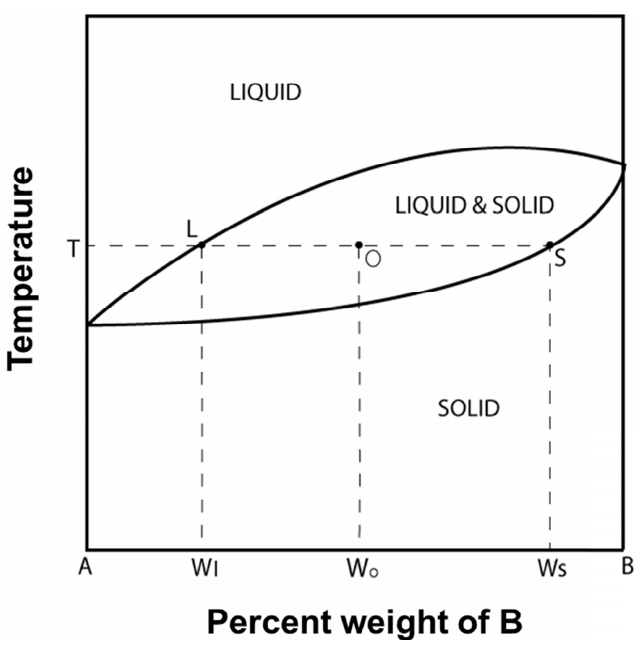
Let us apply the above-mentioned relationship between temperature and mass to changes in morphologies and microstructures in the Fe–C phase diagram according to temperature [8] (Fig 2a). The original x-axis shows the compositional changes of Fe and C; however, if the x-axis becomes the temperature axis, the phase diagram is as shown in Fig 2b. This can be interpreted as an equilibrium composition with respect to temperature. That is, it is the equilibrium mass energy corresponding to a particular space energy. At this point, observing the green points in Fig 2b, it is possible that the simultaneous mixing of Fe and C does not correspond to temperature on a one-to-one basis. However, even if the two elements are mixed, the contents of Fe and C are different at each temperature, and the composition is determined using the lever rule [16] (Fig 3). That is, each temperature has its own composition. Thus, considering a mass basis, it can be seen that different mass energies, according to composition, have corresponding spatial equilibrium energies. Specifically, the main structures in agreement with temperature are as follows [8] (Fig 1b):

(1) The austenite (γ) phase of the face-centered cubic structure, which is stable between 727 and 1493 °C, below 2.14 wt% C

(2) The ferrite (α) phase of the body-centered cubic structure, which is stable up to 912 °C, below 0.022 wt% C

(3) A mixed phase of austenite (γ) and cementite (θ), which is stable between 727 and 1147 °C, with C content above 2.14 wt%

(4) A pearlite phase consisting of ferrite (α) and cementite (θ), which is stable below 727 °C, with C content above 0.022 wt%

These results show that the spatial energy at each temperature corresponds to the mass energy, which changes in each phase to maintain the energetic equilibrium between the two terms.

2.3 Non-equilibrium spatial energy–mass energy relation

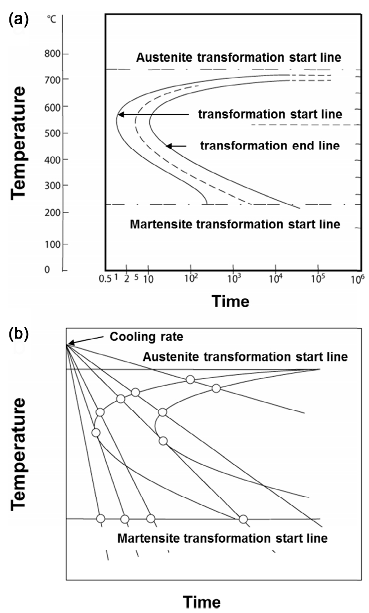
In the previous section, we examined the temperature and phase based on the equilibrium state of Fe–C. However, as is already known, new structures of bainite [17] and martensite [18] can be obtained, depending on the cooling conditions, (i.e., how the temperature is controlled), although not in the equilibrium state (i.e., the phase diagram). These phases can be observed in a separate time-temperature-transformation (TTT) curve [19] (Fig 4a) or a continuous cooling transformation (CCT) curve [20] (Fig 4b).

What is interesting here is that the same austenite phase has caused a bainite or martensite transformation, instead of a ferrite or pearlite transformation. In other words, the cause (austenite source) is the same, but the results (phases) are different. Therefore, from the present point of view, when one state (ferrite or pearlite) is fixed as the equilibrium basis, the other one (bainite or bartensite) becomes the non-equilibrium basis. The possible phase changes are explained as follows:

(1) At relatively high temperatures, it is possible to atomically diffuse into the ferrite or pearlite phase with time.

(2) It is difficult to atomically diffuse into the equilibrium phase with time at relatively low temperatures, which may result in a non-equilibrium bainite or martensite transformation.

If so, as described above, are these non-equilibrium phases able to remain static and stable in a dynamic unstable state? If not, like the half-life [21] of a radioactive element, do they change to ferrite or pearlite, which are equilibrium phases, with time? It is difficult to provide a clear answer to these two questions. This is because, ultimately, maintaining an energetically unstable state is not feasible. Furthermore, no results have been reported to date indicating that bainite or martensite phases have transformed to ferrite or pearlite phases.

This phenomenon can be interpreted as follows. As mentioned earlier, space energy and mass energy always try to maintain equilibrium, and in general, each temperature has an equilibrium state corresponding to the material. As an easy example, in the case of water, water below 0 °C s is present as a solid; from 0 up to 100 °C, it is a liquid, and above 100 °C, it exists as a gas. At this time, the boundary between water and space has an unusual physicochemical property different from existing water and existing space because this is the area where mass and space with different energies achieve energy equilibrium. In other words, boundaries, surfaces, and interfaces can be seen as having both mass and space, and they are the points where the two different energies are uniquely equal. Hence, the implications of the boundary itself can be seen as sharing different parts.

Therefore, since the difference between two energies must be minimized at the boundary, it can be expressed as a mean value, such as (a + b) / 2 = c, where a and b correspond to the respective energies (of mass and space), and c corresponds to a boundary energy. Based on these facts, the bainite and martensite phases, which are not shown in the present equilibrium diagram, can be said to maintain energy equilibrium based on the mass–space energy conservation law. In other words, as shown in Figs 1, 2, 4, whatever the phases are, the appearance of a boundary means that the energies of the symmetrical factors are balanced equally.

Here, the difference in morphology is only the difference between the energy of each space or mass and the original equilibrium energy at which the space and mass show a one-to-one correspondence. Namely, whether the energy difference between mass and space is small or large, it is evident that it is equally a space-mass energy equilibrium.

Therefore, the larger the space-to-mass energy difference, the higher the energy equilibrium at the boundary will be. For this reason, in the case of martensite formed by quenching with a large temperature difference, the energy at the surface is high and the hardness of the steel increases. That is, martensite is not a phase with energy non-equilibrium but one with an energy equilibrium where there is a large difference between the initial spatial energy and mass energy.

2.4 Heat treatment types and energy balance

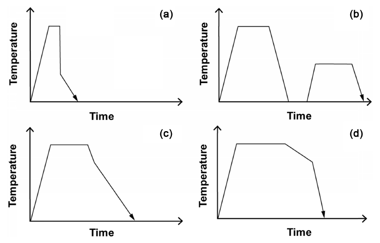
Even though the mass–space energy equilibrium is not elaborately discussed, the heat treatment [22] of metals has long been studied empirically in efforts to improve their mechanical properties, processability, and physical and chemical properties before the effects of heat treatment were scientifically proven [23,24]. However, various types of heat treatments, such as quenching and annealing, are derived from the viewpoint of mass–space energy equilibrium. In other words, they can change mass energy by changing spatial energy through changes in the heating temperature, holding time, and cooling rate. The most commonly used types of heat treatment methods are quenching [25,26], tempering [27,28], normalizing [29,30], and annealing [31,32], and the rough process conditions for these heat treatment methods are shown in Fig 5. The purpose of these various heat treatments can be analyzed in terms of the space-mass energy equilibrium as follows.

(1) Quenching: In this method for increasing the hardness and strength of steel, the difference between the spatial energy and mass energy, is too large as mentioned above. Therefore, only the surface of the mass can become thick and hard because the energies are concentrated at the surface (Fig 5a).

(2) Tempering: To compensate for the brittleness caused by quenching, internal stress, accumulated upon reaching equilibrium, is eliminated; the material becomes tough by cooling in air after heating to a temperature below the transformation point (< 723 °C). In other words, the equilibrium attained during quenching (from the large difference between space energy and mass energy) disappears (Fig 5b).

(3) Normalizing: The steel is heated to the austenite temperature and then air-cooled. This heat treatment is capable of reducing the deformation caused during quenching. The difference between the mass and space energies is usually considered to be in between that of quenching and annealing (Fig 5c).

(4) Annealing: The steel is heated and cooled in the furnace. Since the energy balance is such that the difference between the space energy and mass energy is the smallest, the probability of stress accumulating inside and outside the material is the least (Fig 5d).

Based on the above discussion, it is necessary to clarify that many amorphous materials [33], antimatter [34], and supersaturated [35] and supercooled [36] materials, which are currently defined as non-equilibrium materials, are non-equilibrium materials with respect to only one fixed criterion among various criteria. In principle, according to the major premise of the space–mass energy conservation law, it is reasonable to assume that all the states of the continuum material are energy balance states. Thus, just as mass can be controlled through space, bidirectional energy transfer that can control space through mass will be possible.

3. Conclusions

As spatial energy always has to be in equilibrium with mass energy, the difference between the initial spatial energy and mass energy causes various other physicochemical phenomena inside and outside of materials. The correlation between these two energies is objectively and logically explained via (1) one-to-one correspondences between the equilibrium and non-equilibrium phases based on the phase diagram and (2) the heat-treated Fe–C phases, with the spatial energy represented by temperature. In other words, the states of many materials, which are currently defined as nonequilibrium, have been studied from a narrow viewpoint based on only one fixed criterion. From an integrative point of view, the unchanging states of all materials satisfy the space–mass energy conservation law. The fact that energy can transfer between mass and space and vice versa to achieve equilibrium will surely be a significant factor influencing scientific and technological developments.

Notes

Data Availability

All the data are available from the corresponding author on reasonable request.

Acknowledgments

This research was supported by Basic Science Research Program through the National Research Foundation of Korea (NRF) funded by the Ministry of Education (NRF-2020R1I1A1A01067825 and NRF-2019R1A6A1A11055660). We are grateful to Jiye Kim, Mun Young Koh, Baro Jin, Ha Jin Na, and Koh Eun Na for their cordiality and hospitality during the course of this research.

Notes

Competing interests

The authors declare no competing interests.

Fig. 1.

Existing and new perspectives on energy equilibrium. (a) Gibbs free energy according to the existing energy equilibrium perspective. (b) a collection of consecutive images at a given time showing the new energy equilibrium concept.

Fig. 2.

Two different perspectives on energy balance in the Fe–C phase diagram. (a) The equilibrium phase diagram and corresponding equilibrium microstructure in the conventional binary system composition. (b) The change of each phase and the corresponding microstructure with respect to temperature interpreted as the equilibrium between space energy and mass energy.

Fig. 3.

Whether based on composition or temperature, the lever rule states that each temperature has its own composition. There is a one-to-one correspondence because composition and temperature change at each instant. (percent weight at the S point (X_s) = (W_o – W_l) / (W_s – W_l), percent weight at the L point (X_l) = (W_s – W_o) / (W_s – W_l))

Fig. 4.

TTT and CCT curves as criteria for non-equilibrium transformation. (a) A time–temperature–transformation (TTT) curve as an isothermal transformation curve including both a transformation start line and transformation end line. (b) A continuous cooling transformation (CCT) curve showing the start and end of transformations depending on the cooling rate.

Fig. 5.

In each of the heat treatment methods of steel, a graph shows the heat treatment temperature, holding time, and cooling rate with respect to time. (a) quenching; (b) tempering; (c) normalizing; (d) annealing.

REFERENCES

1. J. Wang, K. Liu, R. Xing, and X. Yan, Chem. Soc. Rev. 45, 5589 (2016).

2. P. Skrzypczyk, A. J. Short, and S. Popescu, Nat. Commun. 5, 4185 (2014).

3. S. Zhou, Phys. Chem. B. 108, 3017 (2004).

4. A. E. Pomerantz, J. P. Camden, A. S. Chiou, F. Ausfelder, N. Chawla, W. L. Hase, and R. N. Zare, J. Am. Chem. Soc. 127, 16368 (2005).

5. C. Kalidas, G. Hefter, and Y. Marcus, Chem. Rev. 100, X-852 (2000).

6. A. Michaelides, Z.-P. Liu, C. J. Zhang, A. Alavi, D. A. King, and P. Hu, J. Am. Chem. Soc. 125, 3704 (2003).

7. H. Karabulut, Renew. Energy. 36, 1704 (2011).

8. H. Okamoto, J. Phase Equilib. 13, 543 (1992).

9. L. Masanes and J. A. Oppenheim, Nat. Commun. 8, 14538 (2017).

10. C. Hess, E. Ozensoy, C.-W. Yi, and D. W. Goodman, J. Am. Chem. Soc. 128, 2988 (2006).

11. M. Racanelli and D. W. Greve, Appl. Phys. Lett. 56, 2524 (1990).

12. S. Yuasa, T. Nagahama, A. Fukushima, Y. Suzuki, and K. Ando, Nat. Mater. 3, 868 (2004).

13. S. Deutschländer, A. M. Puertas, G. Maret, and P. Keim, Phys. Rev. Lett. 113, 127801 (2014).

14. Y. Nakajima, G. J. Li, and T. Tamegai, Physica C. 468, 1138 (2008).

15. J. H. Field, Eur. J. Phys. 35, 055016 (2014).

16. Q. C. Jiang, C. L. Xu, H.Y. Wang, J. G. Wang, and Y. F. Yang, Scr. Mater. 56, 329 (2007).

17. I. A. Yakubtsov, P. Poruks, and J. D. Boyd, Mater. Sci. Eng. A. 480, 109 (2008).

18. T. Ohmura, K. Tsuzaki, and S. Matsuoka, Scr. Mater. 45, 889 (2001).

19. J.-L. Lee and H. K. D. H. Bhadeshia, Mater. Sci. Eng. A. 171, 223 (1993).

20. M.-C. Zhao, K. Yang, F.-R. Xiao, and Y.-Y. Shan, Mater. Sci. Eng. A. 355, 126 (2003).

21. S. Baba, S. Satoh, and C. Yamabe, Vacuum. 65, 489 (2002).

22. B. Varancken, L. Thijs, J.-P. Kruth, and J. V. Humbeeck, J. Alloy. Compd. 541, 177 (2012).

23. H. J. Park, J. H. Lee, B. U. Min, and S. J. Kim, Korean J. Met. Mater. 58, 195 (2020).

24. H.-J. Kim, J. Jung, S.-H. Kim, C.-Y. Lim, and Y. S. Choi, Korean J. Met. Mater. 58, 7 (2020).

25. J. Grum, S. Božič, and M. Zupančič, J. Mater. Process. Technol. 114, 57 (2001).

26. D. V. Edmonds, K. He, F. C. Rizzo, B. C. De Cooman, D. K. Matlock, and J. G. Speer, Mater. Sci. Eng. A. 438-440, 25 (2006).

27. G. Gao, H. Zhang, Z. Tan, W. Liu, and B. Bai, Mater. Sci. Eng. A. 559, 165 (2013).

28. W.-S. Chang, J. Mater. Sci. 37, 1973 (2002).

29. S. Wei and S. Lu, Mater. Des. 35, 43 (2012).

30. P. Yan, Z. Liu, H. Bao, Y. Weng, and W. Liu, Mater. Sci. Eng. A. 597, 148 (2014).

31. R. Song, D. Ponge, D. Raabe, and R. Kaspar, Acta Mater. 53, 845 (2005).

32. H. Luo, J. Shi, C. Wang, W. Cao, X. Sun, and H. Dong, Acta Mater. 59, 4002 (2011).

33. A. Hirata, T. Ichitsubo, P. F. Guan, T. Fujita, and M. W. Chen, Phys. Rev. Lett. 120, 205502 (2018).

34. A. Kusenko, L. Pearce, and L. Yang, Phys. Rev. Lett. 114, 061302 (2015).

35. S. Bengaluru Subramanyam, V. Kondrashov, J. Rühe, and K. K. Varanasi, ACS Appl. Mater. Interfaces. 8, 12583 (2016).

36. S. Lv, M. Cao, C. Li, J. Li, J. Qiu, and S. Zhou, ACS Appl. Mater. Interfaces. 9, 20664 (2017).